This project was part of my honours thesis. The following information is taken from the repository for my honours project:
05/06/2021
Getting SLiM and R to speak to each other
really is not as easy as I thought it would be
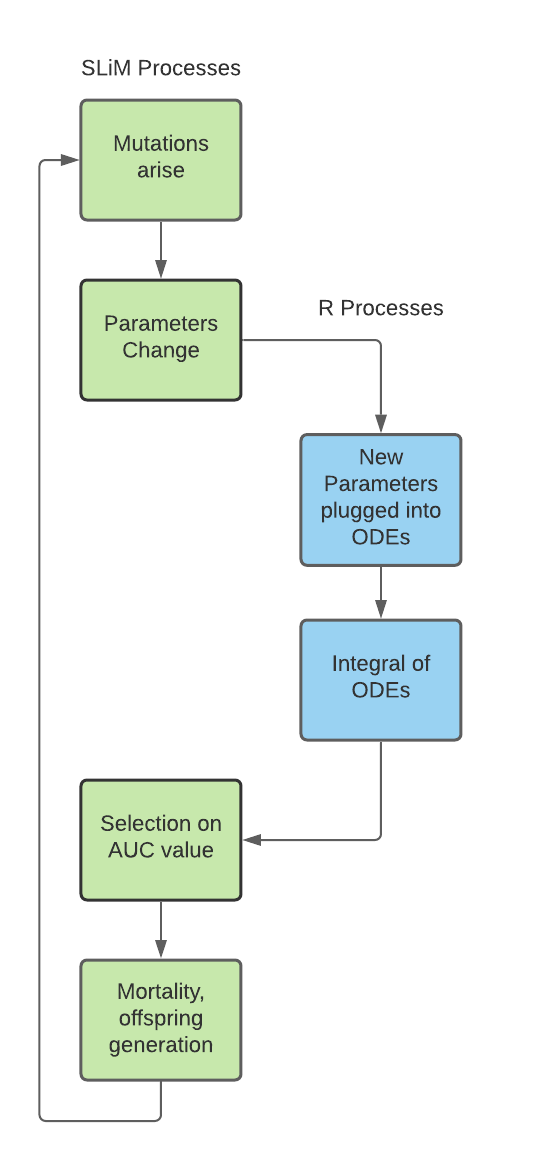
At the heart of this project lie the differential equations that describe the interaction strength between nodes in our simulated genetic networks. These differential equations consist of three key parameters (alpha, beta and the hill coefficient), each of which are acted upon by mutations to change the value of these parameters. This in turn then changes the ODE and thus regulates the amount of subsequent protein produced through a change in interaction strength. My model needs to not only solve these ODE's, but I am also relying on the integral of each function (in other words: the area underneath the curve that these ODE's produce) as to have selection act upon a singular factor rather than act on all three parameters separately (for the sake of computing and my own sanity).
SLiM, while brilliant in its own right, is not capable of solving ODEs, which means I turned towards R, hoping to use the deSolve package. The idea was that SLiM could produce the needed parameter values that had been changed by mutations and these are then fed into R, plugged into the ODEs and the output of those calculations is then fed back into SLiM in order for selection to act upon the individuals. Here in the NAR model, the trait that is selected upon is the concentration of final output produced, which is able to be proxied using the AUC of the interaction between node A and B.
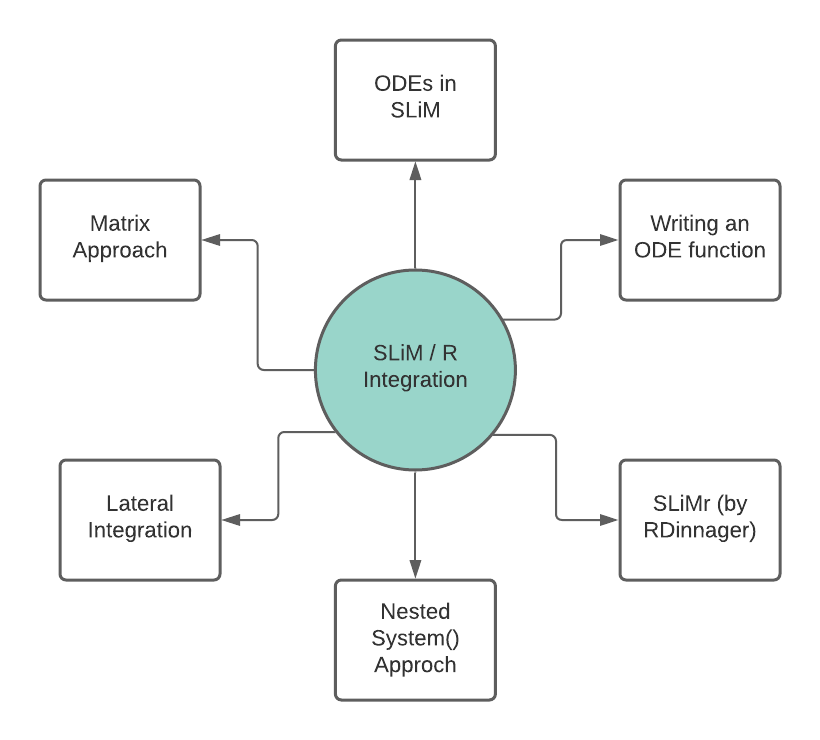
While this sounds simple in principle, it has been a journey trying to get this workflow to work. In total, I have worked through 6 different methods in order to obtain my ODE results:

| Method | Description | Outcome |
|---|---|---|
| ODEs in SLiM | Using SLiM to solve ODEs natively | FAILED, as SLiM has no native ODE function |
| Writing an ODE function | Writing my own eidos function | FAILED, as SLiM lacks the framework to solve ODEs in its current state, as tested and confirmed by Ben Haller |
| SLiMr by RDinnager | Running SLiM from RStudio | FAILED, as these simulations cannot be interrupted by R code, thus lacking the vertical integration I was chasing |
| Nested System() Approach | Nesting an R script in SLiM using the system() function | REJECTED as the output produced was finnicky and feeding the output back into SLiM failed repeatedly due to the constraints of having to use .txt files. Probably could have been able to get this to work, but it seemed not worth the trouble |
| Lateral Integration | Running SLiM and R in parallel in a tight circuit | VIABLE after extensive testing, originally thought to be FAILED as well. Relies on the export and import of singleton text files that end up producing float vectors in SLiM. May be computational inefficient for larger models. |
| Matrix Approach | Developing matrices of individual barcodes, mutation vectors and pre-calculated ODE solutions which are then all fed into SLiM. R is used to generate these matrices but is not active during the simulation run | POTENTIALLY VIABLE, I have yet to test if SLiM can match and call values from different matrices as the matrix support within SLiM is essentially a worser version of the R matrix support, as all matrices remain vectors within the SLiM scope. I have been working on the code to create these matrices, as this may prove to be computationally more efficient especially for larger models. |
Essentially, the majority of my work in April and May has been working through these six approaches and attempting to integrate SLiM and R. This goes hand in hand with trawling through both the SLiM and Eidos manuals and learning nested and parallel coding structures.
While most of these six approaches are not viable for my project, there are three approaches which remain interesting in their own right. These were the approaches that I have spent most time on and I would recommend to other researchers that are interested in integrating SLiM and R or would like to extend the functionality of SLiM.
SLiMr : Powerful for code optimisation
SLiMr is a package for R developed by RDinnager, which essentially allows the user to write and run SLiM scripts from R or RStudio. The true power of SLiMr lies in it's slim_inline() function, which allows the user to define a vector of values that should be used in subsequent runs of the slim model, without having to go in and change the code each time. It also allows the user to create output that is formatted so that R can immediately use it without the need to tidy or reformat slim output.
- slim_inline() is very useful for creating replicates easily
- slim_outline() allows for quick tidy data
- superb choice if you need base SLiM functionality and would like to conduct R analysis
- cannot run R code within your simulations* so there is no true Integration
- documentation and debugging is still in the works
*SLiMr is still being developed, so its functionality may have expanded by the time I have finished uploading this readme, so take the fact that it has been rejected for this project as a product of the time I have worked on it.
Lateral Integration
Lateral integration, in my books at least, refers to the fact that SLiM and R are running in parallel for the entirety of these SLiM simulation. Each generation, SLiM writes to a file which is read by R, R then writes to another file and this file is read in by SLiM and acted upon by SLiM. This is an incredibly powerful approach to working with SLiM and can be extended to any software that can write to .txt, not just R.

There are some basic ground rules, but essentially, as long as you can create a text file with the numeric output that you need, you can use lateral integration to work with any other supplementary programme. It is important to note that only singleton files may be read in (ie a file that contains one row of "1 2 3 4 5" and not a file with two rows in the format of "1: 1 2 3 4 5, 2: 6 7 8 9 10"). Similarly, these text files have to be space-separated and must not contain whitespace after the last number, otherwise SLiM will throw an error message.
The basic code to use this approach is:
x = readFile("~/Desktop/file.txt");
x = asFloat(strsplit(x));
It is imperial that you use the strsplit() function, as SLiM will otherwise not recognize that there are multiple data entries within your text file.
If you would like to check that everything worked the way it should, here is some test code taken from my own project:
	IDS = readFile("~/Desktop/test.txt");
	IDS = asFloat(strsplit(IDS));
	print("These are your individuals here:");
	print(IDS);
	val = isFloat(IDS);
	print("TRUE OR FALSE that we all  FLOAT down here?:" + val);
This should print your file content and the isFloat() should return T.
With lateral integration, you can then manipulate your data like any other float vector within SLiM (for example, cbind() it to another imported text file if you need to make a matrix or a data frame within SLiM!).
- allows input from ANY programme that can export text files
- output can be generated and used within each generation
- huge potential to expand SLiMs functionality (especially mathematically)
- may be computationally expensive as it requires continues writing to file
- only supports singleton text output, so full dataframes are time intensive to recreate
This approach is my preferred approach to creating the NAR model, and is the one I am currently (04/06) working on.
The Matrix Approach
The Matrix approach essentially eliminates the need to use R within the simulations, and instead relies on the complete availability of all possible outcomes before the simulation even begins. This process relies on three matrices:
- The Barcode Matrix, abbreviated B, which takes the number of basepairs of each focal gene and creates all possible binary combinations, i.e. 00000 or 00100 or 01010, etc.
- The Mutations Matrix, abbreviated M, which is a 1:1 copy of B except that it replaces all incidences of 1 in the barcode matrix with a random mutational effect size. This may be drawn from a normal distribution, a gaussian distribution or any other distribution that best fits your model.
- The Parameter Matrix, abbreviated P, where all the effect sizes that represent a parameter of interest are summed with the initial parameter value for that model run. This matrix exists just for the user's convenience, as it allows you to take all mutations that pertain to one parameter and see the overall net effect on this parameter. This step assumes additivity of mutational effects WITHIN a gene (whereas the model assumes non-additivity across genes).
- The ODE Matrix, which is a matrix that contains all ODE solutions that correspond to each barcode. These solutions are calculated using M and P.
Note that M, P, and ODE matrices are all unique for each model run. Each model run in turn consists of multiple simulation seeds; i.e. the seeds are the replicates for each runs.
These matrices are all fed into SLiM at the start of each simulation and SLiM refers and cross-references these matrices to obtain mutational effect sizes and have selection act upon the final ODE values - in theory. This has not been tested yet, so this methodology remains only POTENTIALLY VIABLE.
- computationally efficient and inexpensive
- Matrices can be easily generated using R
- Full control over input in simulation
- Untested, SLiM may still struggle with cross-referencing
- Need to create barcode matrices and all data upfront may limit the size of genes modelled (ie 10 basepairs rather than 1000)
Moving forward
I will be working with my lateral integration approach, and potentially further research and develop the matrix approach. I hope this guide serves as a useful tool for other researchers that would like to use/manipulate/expand SLiM in a similar fashion.
Credit is highly appreciated. Stella Knief